Capacity and Demand Extremes: Managing Risk of Failure 

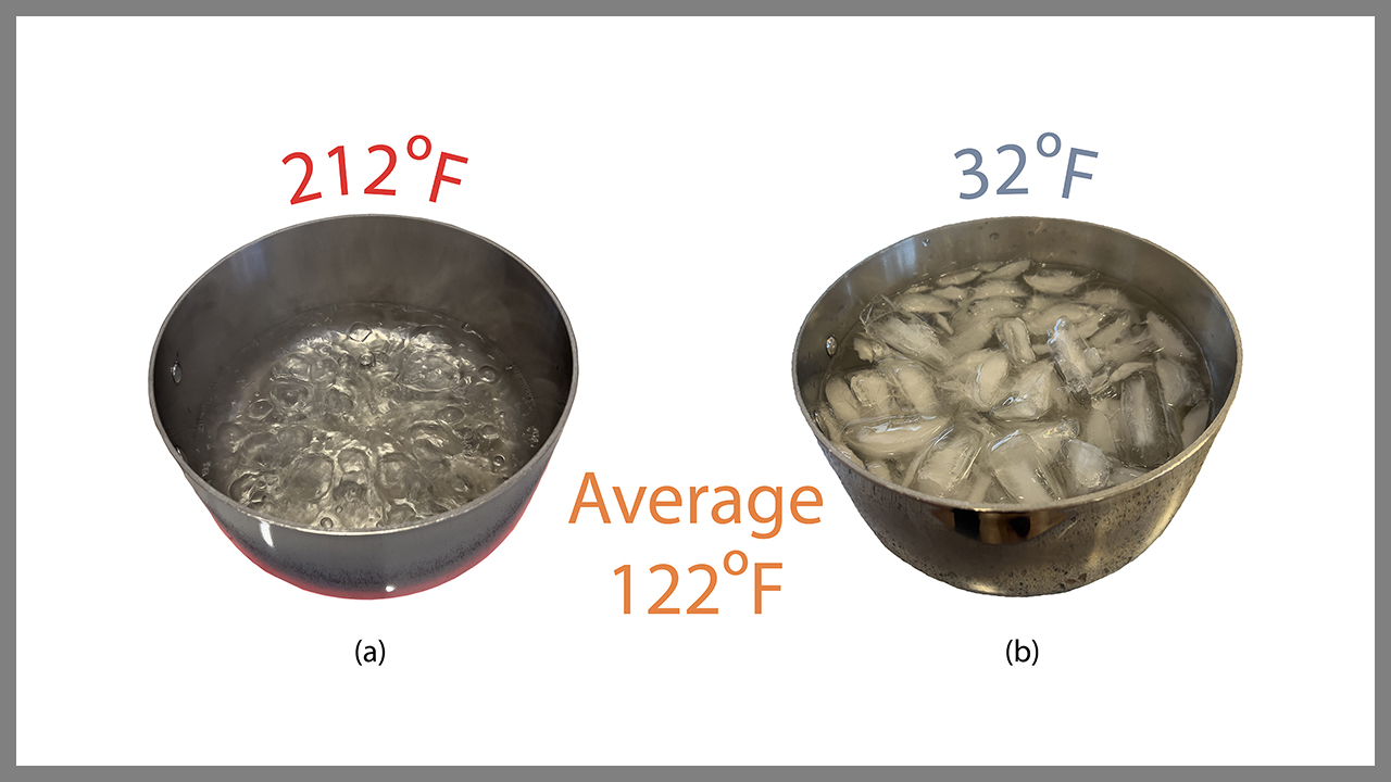
Figure 1. I’m at risk of serious injury placing one hand in boiling water (a) and the other in nearly freezing water (b), even though on average my hands would just be uncomfortably hot at 122 degrees. Mitigating the failure risk of engineered systems responds to similar concerns in that we must assess outcomes from the least favorable capacity-demand interactions rather than the average interactions.

RAILWAY AGE, SEPTEMBER 2023 ISSUE: Welcome to “Timeout for Tech with Gary T. Fry, Ph.D., P.E.” Each month, we examine a technology topic about which professionals in the railway industry have asked to learn more. This month we focus on managing the risk of failure of engineered components.

I am often asked about the methods engineers use to mitigate the risk of failure of systems that we design and manufacture. To begin, it is important to know that there are two distinct phases of “system life” to consider: Phase 1—ensuring an acceptably low risk of failure of a brand-new system and Phase 2—ensuring an acceptably low risk of failure of an operating system in service.

Phase 1 is the culmination of system planning, design, and manufacturing activities. Phase 2 comprises sustained support of the system in service and includes four activities: (a) data collection through system inspection and performance monitoring; (b) data-driven evaluation of system safety and functional adequacy—i.e., fitness for service; (c) system owner’s strategic planning and decision-making protocols; and (d) system owner’s deployment of resources for system maintenance, repair, retrofit, and/or replacement.

Both phases usually include statistical analyses to determine a system’s fitness for service. In general, an engineered system fails whenever the demand placed on the system exceeds its capacity. Alternatively, we could define failure as occurring whenever the capacity of a worn system falls below the demand required of it. Therefore, a key part of any fitness for service assessment is to estimate the system’s current, in situ capacity and to estimate the demand placed on the system. If, by an acceptable margin, the system’s estimated capacity exceeds its estimated demand, the system is deemed “fit” for service. If not, the system is prioritized for remediation.

As a concept, fitness for service is logical and intuitive. But there are nuances in the details that deserve more discussion. Here, we will focus on the terms estimated capacity, estimated demand, and acceptable margin. When a capacity or a demand is provided as an estimate, rather than as an exact number, some uncertainty is involved. There exists some range of values within which the estimate falls. So, one way to approach the issue is to use estimates for the averages of capacity and demand. If the average capacity exceeds the average demand by a comfortable margin, one might argue that the system is fit. Though this might seem to be a legitimate strategy, it is not a recommended approach because it can lead to undesirable consequences. To understand why, refer to Figure 1 (above).

Figure 1(a) is a photograph of a pot of boiling water. Figure 1(b) is a photograph of a pot of icy water. Let’s consider this range of water temperatures as an example of demand. We can estimate that the average demand might be 122 degrees Fahrenheit. Now consider that the system under that demand is my bare hand performing a service that requires it to be submerged periodically for two seconds.

The 122-degree average demand is hot for my skin, but it’s tolerable for at least six seconds—three times as long as required. Even with this “factor of safety” of three, however, I should not conclude that my bare hands are fit to serve in this scenario. Simply put, the average demand does not reveal the possibility of boiling hot water at the extreme end, which will cause serious burns in less than a second. This simple example illustrates clearly why fitness for service determinations cannot rely on average capacity and demand values.

Instead, minimum capacity and maximum demand extremes must be managed over the full life of an engineered system. For example, when a new engineered system is placed into service (Phase 1 of the system’s life), the planning, design, and manufacturing processes are established to provide a high confidence level that the extreme values of capacity and demand will interact desirably. In fact, there are usually international standards, specifications, codes of recommended practice, and local jurisdictional requirements that affect, and even define, the quantitative relationships between capacity and demand of a newly minted system.

It is most often during Phase 2 of the system’s life, under the effects of normal wear and tear, which often includes fatigue damage accumulation and possible increases to the demand environment that systems present with increased risk of failure. And it is the policies and procedures of the systems’ owners that determine the extent to which the risk of failure increases. Notably, two identical systems that are exposed to identical service environments but are managed by two different owners may develop different risks of failure over time that reflect the different owner’s policies and procedures—particularly those described as Phase 2(c) and Phase 2(d) earlier.

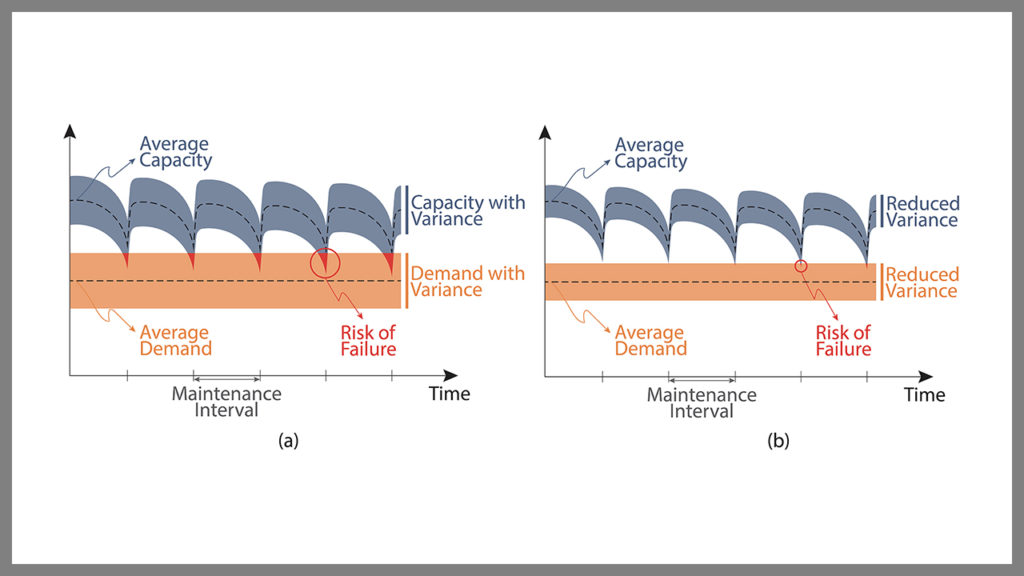
For example, consider Figure 2 (above). Figures 2(a) and 2(b) illustrate the capacity and demand statistics for two identical inventories of systems—each managed by a different owner. In each case, the inventories experience relatively constant ranges of demand against capacity ranges that vary substantially over time. Each figure illustrates a representative window of Phase-2 inventory performance as its systems experience expected deterioration, such as fatigue defects in railway wheels and rails. The figures also illustrate the effects of periodic repairs and/or replacements over routine maintenance intervals. The owners observe failures whenever the capacities of the weakest systems in their inventories fall below the peak demands.

It is very important to note that the capacity and demand ranges are smaller in Figure 2(b). At all times, however, the average capacities in Figures 2(a) and 2(b) are identical to one another and remain well above the average demands, which are also identical between the two figures. The only differences between the two figures are the ranges of values for capacity and demand.

To build their inventories, both owners purchased the same systems from the same suppliers. Subsequently, they managed their inventories differently. The owner of the inventory illustrated in Figure 2(b) maintained it in such that capacity and demand ranges were smaller, thereby achieving a substantially lower probability of failure than the owner of the inventory in Figure 2(a).

The takeaways are these:

• Failures of engineered systems generally occur during Phase 2 of the systems’ life cycles. The usual failure scenario occurs when a weaker-than-average system is subjected to a higher-than-average demand.

• System management policies that maintain capacity and demand ranges within target bandwidths can effectively control system failure risks by limiting the most disparate extreme value interactions between capacity and demand. In doing this, the weakest components in service are less weak and the highest demands in service are lower. This is true even when average capacity and demand values do not change.

Dr. Fry is Vice President of Fry Technical Services, Inc. He has 30 years of experience in research and consulting on the fatigue and fracture behavior of structural metals and weldments. His research results have been incorporated into international codes of practice used in the design of structural components and systems, including structural welds, railway and highway bridges, and high-rise commercial buildings in seismic risk zones. He has extensive experience performing in-situ testing of railway bridges under live loading of trains, including high-speed passenger trains and heavy-axle-load freight trains. His research, publication, and consulting have advanced the state of the art in structural health monitoring and structural impairment detection.