Managing Failure Risk
Written by Gary T. Fry, Vice President, Fry Technical Services, Inc.; Railway Age Contributing Editor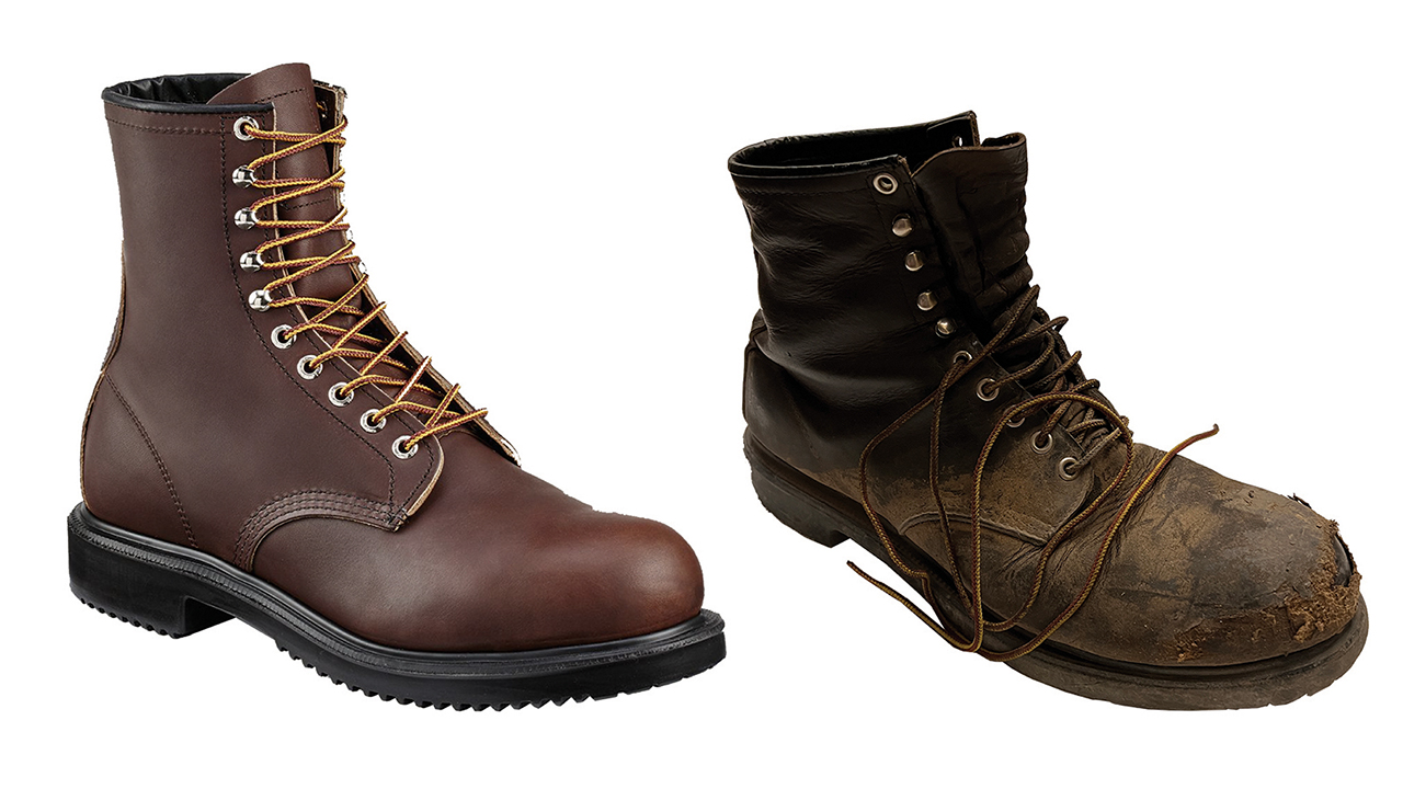
Figure 1. Photograph of two boots illustrating a new system vs. an old system nearing the end of its useful service life. (Courtesy of Gary T. Fry.)
RAILWAY AGE, JUNE 2022 ISSUE: Welcome to “Timeout for Tech with Gary T. Fry, Ph.D., P.E.” Before we begin, I want to highlight an upcoming RT&S virtual technical conference that will convene on July 14, 2022. The conference theme is Track Geometry and Friction Management. I will be participating and presenting on the “Benefits of Geometry Measurement Automation and Trending.” The full conference program and registration details are available online at https://www.railwayage.com/track-geometry/. I hope you will join us!
Each month in this ongoing series, we examine a technology topic that professionals in the railway industry have asked to learn more about. This month, we discuss strategies to manage risk of failure. Obviously, this topic is very broad and has applications in every kind of business endeavor and in our everyday lives as well. Narrowing things down a bit, we will focus on the performance of aging engineered systems and specifically on managing the risk of failure of load-bearing components, such as steel rails and steel wheels, that are nearing the end of their intended service lives.
To get started, let’s consider a simple example of a system that exhibits wear and tear and deterioration with use. Figure 1 is a photograph of two steel-toed work boots—one unused and the other clearly near the end of its useful life. If the boot manufacturer follows a strict quality control program, we would expect that the unused boot is representative of the general population of new boots of that model. We hold this expectation because we assume the quality control program results in a narrow bandwidth of variability among a large population of new boots.
What about the boot near the end of its life in Figure 1? If we were to inspect a large sample of boots of the same age as the used boot, it is likely that we would observe wide variability in condition. Some might be like-new and barely used at all, while others might be in worse shape than the used boot in the photo. Because of this variability, a used boot selected to be in average condition for the age group would not be reasonably representative of either the best boots or the worst boots.
We encounter this same type of problem when assessing load-bearing components of engineered systems. When the components are new, the variability of critical properties has been controlled during manufacture to fall within an acceptably small range among a large population of components. But once the systems have been in use, the variability in properties increases.
The main concern with aging load-bearing components is the potential that they have become weaker after prolonged exposure to repetitive loads and to their surrounding environments. Some of the components might become weaker because of corrosion that reduces the amount of material available to resist load. Some of the components might become weaker because they have developed fatigue cracks that give rise to the potential for sudden fracture under load. It is also possible that some of the components are minimally weakened. Essentially then, the effect of time-in-use has been to increase the uncertainty of the capacity of the components.
Figure 2 is a plot of frequency distributions for capacity and demand of load-bearing components in an engineered system. One demand curve is shown and is assumed representative over the 40 years of evaluation of the systems. Five capacity curves are shown representing a new system and a system after increasing years of service exposure: 10 years, 20 years, 30 years and 40 years.
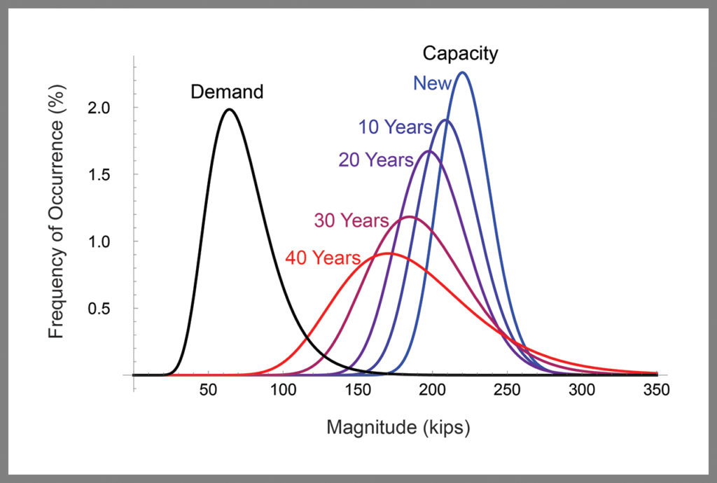
After each decade of service, we observe a slight decline in average capacity: average capacity values shift to the left. However, the average capacity value, even after 40 years, remains well above the average demand value—by a factor of more than 2.5. Of more concern is the notable increase in variability about the average: The capacity curves become wider.
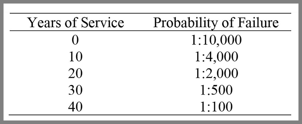
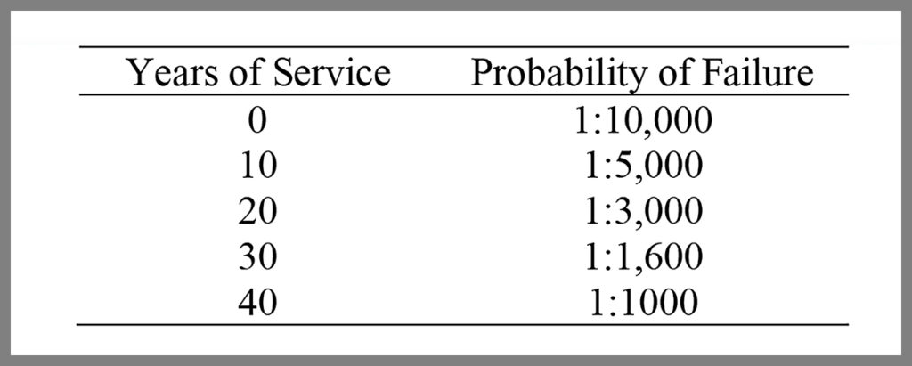
Now, let’s look at what has happened to the probability of failure of these systems after each decade. Table 1 lists the probabilities of failure for each of the five capacity curves. When the systems are new, the probability of failure is roughly 1 in 10,000. After 40 years, the probability of failure has increased to 1%, that is, by a factor of 100.
Now, let’s look at the effect of managing these systems differently. Specifically, imagine that we introduce inspection and maintenance policies designed to keep the variability of the capacity of the systems roughly constant over time and nearly the same as when they were first installed. We will not attempt to control the average values of the capacities, allowing them to shift lower as observed in Figure 3. To accomplish this strategy, we remove components from service that are assessed as falling below a threshold capacity, and repair them or replace them.
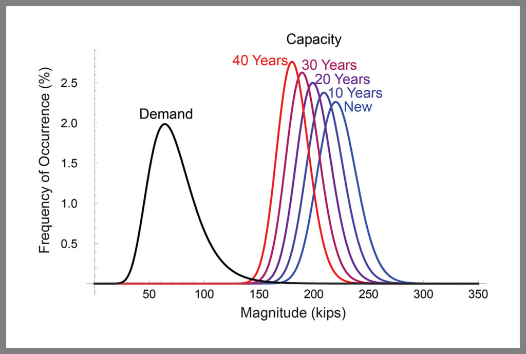
Figure 3 shows a plot of the frequency distributions that result from our proposed inspection and maintenance strategy. We observe the same reductions in average values with each decade of service as before, but now the variability is constant.
Table 2 shows the effect of this approach on probability of failure of the systems. As before, the probability of failure of new systems is roughly 1 in 10,000. But now the probability of failure after 40 years is 1 in 1,000, which is improved by a factor of 10 compared with the previous case.
To manage the risk of failure of load-bearing components in engineered systems, we must inspect the components, assess their capacity, and repair or replace them according to a defined policy. As straightforward as this sounds, there remains a challenging question: When should a component be repaired or replaced?
A logical end goal is to ensure that the probability of system failure always remains acceptably low. One very effective management strategy for this is to control the variabilities of demand and capacity statistics.

Dr. Fry is Vice President of Fry Technical Services, Inc. He has 30 years of experience in research and consulting on the fatigue and fracture behavior of structural metals and weldments. His research results have been incorporated into international codes of practice used in the design of structural components and systems including structural welds, railway and highway bridges, and high-rise commercial buildings in seismic risk zones. He has extensive experience performing in situ testing of railway bridges under live loading of trains, including high-speed passenger trains and heavy-axle-load freight trains. His research, publications and consulting have advanced the state of the art in structural health monitoring and structural impairment detection.