Understanding Failure Risk
Written by Gary T. Fry, Vice President, Fry Technical Services, Inc.; Railway Age Contributing Editor
Figure 1. A person trying to lift an object is a familiar example of a system at risk of failing. (Courtesy of Gary T. Fry.)
RAILWAY AGE, MAY 2022 ISSUE: Welcome to “Timeout for Tech with Gary T. Fry, Ph.D., P.E.” Each month, we examine a technology topic that professionals in the railway industry have asked to learn more about. This month, we discuss risk of failure and methods we can use to quantify this risk.
Even after expending our best efforts, in most human endeavors, there is no such thing as “zero probability of failure.” Engineered systems are not exceptions to the rule. Consequently, assessing risk of failure is an essential part of planning, designing, building, operating and maintaining these systems. In particular, the concepts of capacity and demand and their relative magnitudes are the most important objectives to control, especially in the context of ensuring safety. We begin with a familiar example that illustrates the essential features of a typical risk of failure assessment problem.
Figure 1 (above) is a photograph of a person trying to lift a pumpkin. What is the risk that this effort will fail? To answer the question, we need to know this person’s maximal lifting capacity and the weight of the pumpkin. If the weight of the pumpkin exceeds the person’s maximal lifting capacity, we might reasonably conclude that there is a risk of failure approaching 100%. Conversely, if the person’s maximal lifting capacity exceeds the weight of the pumpkin, we assess a risk of failure close to 0%.
Let’s extend this analysis a little by considering two scenarios. First, imagine that one person, who happens to possess a lifting capacity of 25 pounds, enters a yard filled with 10,000 assorted pumpkins that vary in weight. Once inside the yard, he tries to lift one of the pumpkins selected at random. What is the risk of failure?
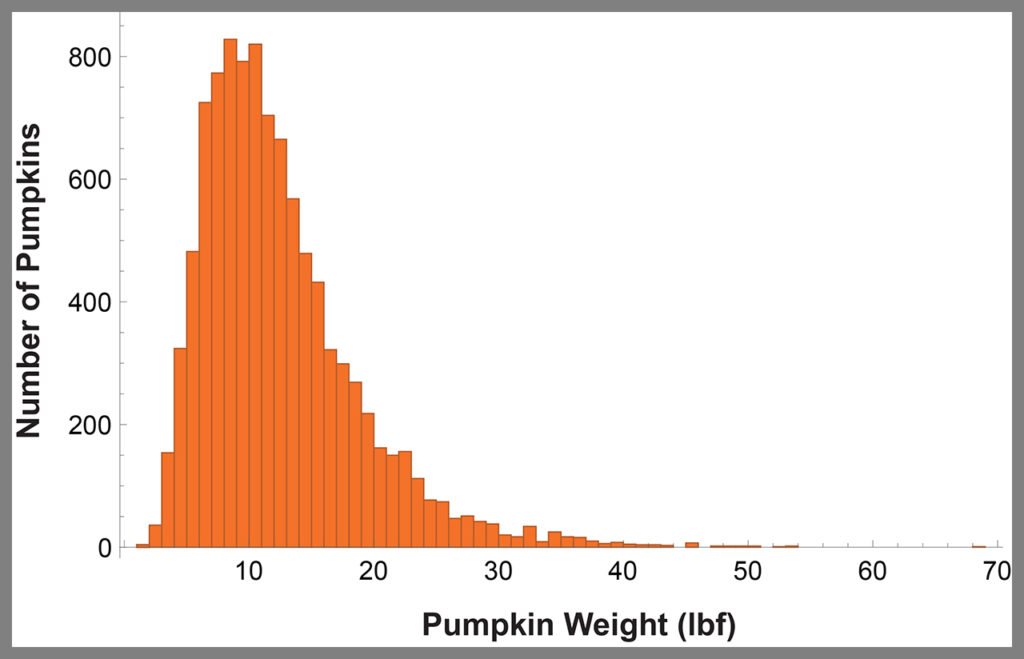
To perform this risk assessment, we need some data regarding the weights of pumpkins in the yard. Figure 2 (below) is a histogram representing the distribution of weights of the 10,000 pumpkins. All we need to do is determine the number of pumpkins that weigh more than 25 pounds (this person’s lifting capacity) and divide by the total number of pumpkins in the yard. In this case, it turns out that there are 472 pumpkins that weigh more than 25 pounds. The result of the calculation gives a risk of failure of 4.7%.
For the second scenario, imagine that a very large group of people, who possess varying lifting capacities, enters the yard. A person selected at random tries to lift one of the pumpkins also selected at random. What is the risk of failure?
This scenario is more complicated than the first, but it is closely related to the types of risk assessments we perform on engineered systems. The large group of people is analogous to a large population of similar engineered systems, such as railway wheels, that because of wear and tear possess varying capacity. The pumpkins are analogous to the varying demand placed on the population of systems, such as the amount and type of material that might be loaded into a railcar.
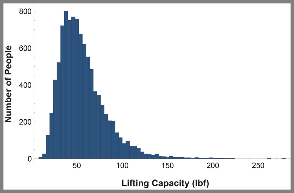
To continue with our risk assessment, we need more data. For example, Figure 3 (below) is a histogram representing the lifting capacity of 10,000 different people. Note that we now have data on 10,000 people and 10,000 pumpkins—one pumpkin for each person.
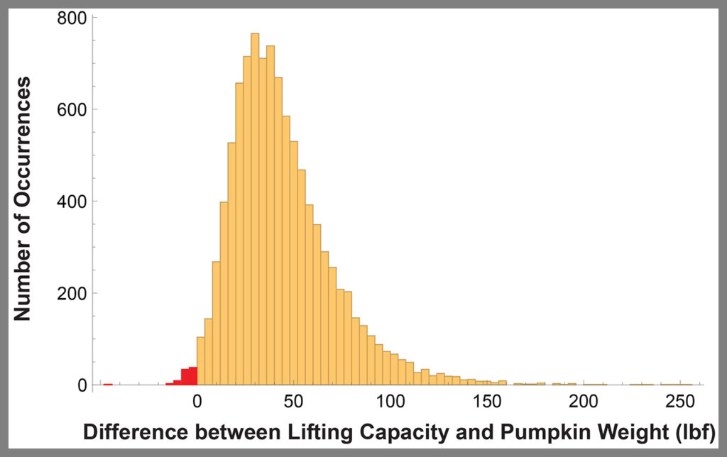
There are a few ways that we can proceed from here that are equally acceptable. Let’s focus on one approach. Select at random, from each of these two data sets, a person’s lifting capacity and a pumpkin weight. Subtract the pumpkin weight from the lifting capacity. The resulting difference is a new data sample to be included in a new data set. Continue this process, without reusing any of the data, until no data pairs remain.
Figure 4 (below) is a histogram that represents a result from applying this algorithm. The differences calculated between 10,000 random pairs resulted in 75 failures that are visible as red-shaded bars plotted left of zero on the horizontal axis. Hence the risk of failure is 0.75%. This process should be repeated, each time randomly selecting one element from each data set to create a random pairing. Each effort will provide a different estimate for risk of failure, and the set of those results will comprise a representative failure statistic. For example, after 10 repetitions, the average risk of failure was 0.85%, which is a little larger than the single initial calculation of 0.75%. The results are different each time because with each new analysis a given capacity might be paired with a different demand since the pairings are done at random. It is often desirable to perform the assessment this way, as we gain some additional insight into the variability present in the problem. Again, there are several ways to approach the problem; each has its merits.
From the previous example, we see that an assessment of failure risk is a problem in statistics. And from the unique perspective of statistics, we can gain insight into the characteristics of a system that give rise to its risk of failing. From that insight, we can develop effective mitigation strategies that control the risk of failure.
Consider Figure 5 (below), which illustrates on a single plot an engineered system’s frequency distributions for capacity (blue curve) and demand (orange curve). We see that the average values of capacity and demand are well separated—by a factor of two. The average value for capacity is 150 tons and the average value for demand is 75 tons. Despite this appreciable separation of average values, however, we also see that the two curves overlap. Hence the magnitudes of some occurrences of demand can be expected to exceed the magnitudes of some occurrences of capacity, which will cause failure of the system. Applying the same algorithm used to solve the second scenario above, the probability of failure of the system represented in Figure 5 is roughly 5%.
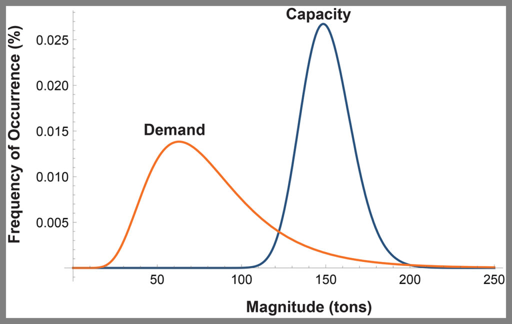
for an engineered system. (Courtesy of Gary T. Fry.)
To understand the risk of failure of an engineered system, it is necessary, at a minimum, to understand the statistical distributions of the system’s capacity and demand variables. Following that, to mitigate risk of failure, it is not enough to simply control and separate the average values of capacity and demand. It is also necessary to control the upper reaches of demand and the lower reaches of capacity.
The objectives are to establish by design and then maintain during operation, an “acceptably low” risk of system failure. Defining an acceptably low risk of failure for a given system is usually very challenging, especially in situations involving life safety. Instinctively, we all want the risk to be zero. In theory, however, a nonzero probability of failure will always exist.

Dr. Fry is Vice President of Fry Technical Services, Inc. He has 30 years of experience in research and consulting on the fatigue and fracture behavior of structural metals and weldments. His research results have been incorporated into international codes of practice used in the design of structural components and systems including structural welds, railway and highway bridges, and high-rise commercial buildings in seismic risk zones. He has extensive experience performing in situ testing of railway bridges under live loading of trains, including high-speed passenger trains and heavy-axle-load freight trains. His research, publications and consulting have advanced the state of the art in structural health monitoring and structural impairment detection.